I spend a lot of time in Excel. It’s not my favorite program in the world.
I frequently run into scenarios where we get a set of data from a customer, run through analysis, then get a new set of data that has more VMs.
In many cases, we’ve already spent hours on the old dataset categorizing VMs – VMs the customer wants to ignore, VMs the customer wants to put into a large cluster like i3en, etc. Many of these sizings contain thousands of VMs.
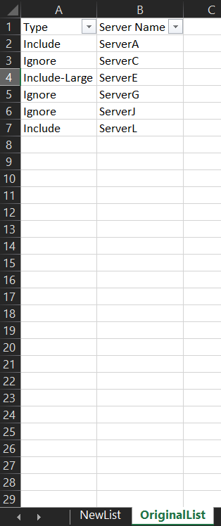
Here is my sample data. In the OriginalList tab, I pasted the data from the workbook that has the first set of VMs that we categorized.
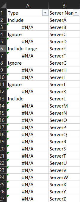
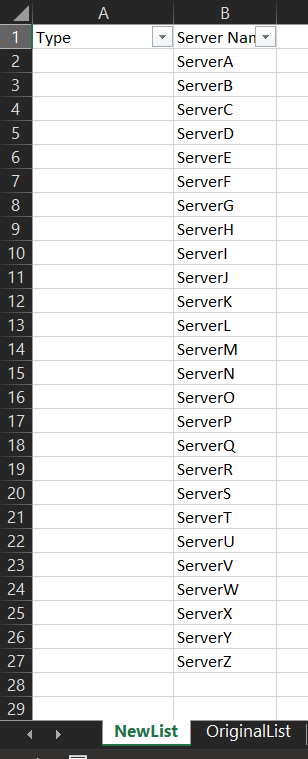
The NewList tab contains a larger list of VMs to simulate a new list with more VMs in it than we originally categorized
This is the formula I used. I spent a lot of time on accounting websites trying to figure it out.
=IF(INDEX(OriginalList!$A$2:$A$27,MATCH(B2,OriginalList!$B$2:$B$7,0)) = 0,””,INDEX(OriginalList!$A$2:$A$27,MATCH(B2,OriginalList!$B$2:$B$7,0)))
Let’s break down the formula. NewList cell B2 contains the value ‘ServerA’. The MATCH statement searches OriginalList column B, rows B2 through B7, looking for the value ‘ServerA’ found in New List cell B2.
If a match is found, the MATCH statement returns the row number where ‘ServerA’ was found. In this case, the MATCH statement returns the value 2.
The INDEX statement then finds the corresponding Type data in Original List Column A, row 2.

I now have a match for A2. To bring the formula down to the rest of the spreadsheet, I double-click on the box in the lower right corner.
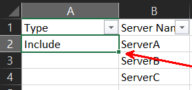
Now I have the OriginalList data in the NewList.